19.6.1.1. Prim’s Algorithm¶

The first of our two algorithms for finding MCSTs is commonly referred to as Prim’s algorithm. Prim’s algorithm is very simple. Start with any Vertex \(N\) in the graph, setting the MCST to be \(N\) initially. Pick the least-cost edge connected to \(N\). This edge connects \(N\) to another vertex; call this \(M\). Add Vertex \(M\) and Edge \((N, M)\) to the MCST. Next, pick the least-cost edge coming from either \(N\) or \(M\) to any other vertex in the graph. Add this edge and the new vertex it reaches to the MCST. This process continues, at each step expanding the MCST by selecting the least-cost edge from a vertex currently in the MCST to a vertex not currently in the MCST.

Prim’s algorithm is quite similar to Dijkstra’s algorithm for finding the single-source shortest paths. The primary difference is that we are seeking not the next closest vertex to the start vertex, but rather the next closest vertex to any vertex currently in the MCST. Thus we replace the lines:

if (D[w] > (D[v] + G.weight(v, w)))
  D[w] = D[v] + G.weight(v, w);

in Djikstra’s algorithm with the lines:

if (D[w] > G.weight(v, w))
  D[w] = G.weight(v, w);

in Prim’s algorithm.

The following code shows an implementation for Prim’s algorithm that searches the distance matrix for the next closest vertex.

// Compute shortest distances to the MCST, store them in D.
// V[i] will hold the index for the vertex that is i's parent in the MCST
void Prim(Graph G, int s, int[] D, int[] V) {
  for (int i=0; i<G.nodeCount(); i++) {    // Initialize
    D[i] = INFINITY;
  }
  D[s] = 0;
  for (int i=0; i<G.nodeCount(); i++) {  // Process the vertices
    int v = minVertex(G, D);     // Find next-closest vertex
    G.setValue(v, VISITED);
    if (D[v] == INFINITY) { return; } // Unreachable
    if (v != s) { AddEdgetoMST(V[v], v); }
    int[] nList = G.neighbors(v);
    for (int j=0; j<nList.length; j++) {
      int w = nList[j];
      if (D[w] > G.weight(v, w)) {
        D[w] = G.weight(v, w);
        V[w] = v;
      }
    }
  }
}

For each vertex \(I\), when \(I\) is processed by Prim’s algorithm, an edge going to \(I\) is added to the MCST that we are building. Array V[I] stores the previously visited vertex that is closest to Vertex I. This information lets us know which edge goes into the MCST when Vertex \(I\) is processed. The implementation above also contains calls to AddEdgetoMST to indicate which edges are actually added to the MCST.

Settings

Saving...
Server Error
Resubmit

19.6.1.2. Prim’s Algorithm Alternative Implementation¶

Alternatively, we can implement Prim’s algorithm using a priority queue to find the next closest vertex, as shown next. As with the priority queue version of Dijkstra’s algorithm, the heap stores DijkElem objects.

// Prims MCST algorithm: priority queue version
void PrimPQ(Graph G, int s, int[] D, int[] V) {
  int v;                                 // The current vertex
  KVPair[] E = new KVPair[G.edgeCount()];        // Heap for edges
  E[0] = new KVPair(0, s);               // Initial vertex
  MinHeap H = new MinHeap(E, 1, G.edgeCount());
  for (int i=0; i<G.nodeCount(); i++) {            // Initialize distance
    D[i] = INFINITY;
  }
  D[s] = 0;
  for (int i=0; i<G.nodeCount(); i++) {          // For each vertex
    KVPair temp = H.removemin();
    if (temp == null) { return; }      // Unreachable nodes exist
    v = (Integer)temp.value();
      while (G.getValue(v) == VISITED) {
        KVPair temp = H.removemin();
        if (temp == null) { return; }      // Unreachable nodes exist
        v = (Integer)temp.value();
      }
    G.setValue(v, VISITED);
    if (D[v] == INFINITY) { return; }  // Unreachable
    if (v != s) { AddEdgetoMST(V[v], v); } // Add edge to MST
    int[] nList = G.neighbors(v);
    for (int j=0; j<nList.length; j++) {
      int w = nList[j];
      if (D[w] > G.weight(v, w)) { // Update D
        D[w] = G.weight(v, w);
        V[w] = v;                  // Where it came from
        H.insert(D[w], w);
      }
    }
  }
}

Prim’s algorithm is an example of a greedy algorithm. At each step in the for loop, we select the least-cost edge that connects some marked vertex to some unmarked vertex. The algorithm does not otherwise check that the MCST really should include this least-cost edge. This leads to an important question: Does Prim’s algorithm work correctly? Clearly it generates a spanning tree (because each pass through the for loop adds one edge and one unmarked vertex to the spanning tree until all vertices have been added), but does this tree have minimum cost?

Theorem: Prim’s algorithm produces a minimum-cost spanning tree.

Proof: We will use a proof by contradiction. Let \(\mathbf{G} = (\mathbf{V}, \mathbf{E})\) be a graph for which Prim’s algorithm does not generate an MCST. Define an ordering on the vertices according to the order in which they were added by Prim’s algorithm to the MCST: \(v_0, v_1, ..., v_{n-1}\). Let edge \(e_i\) connect \((v_x, v_i)\) for some \(x < i\) and \(i \leq 1\). Let \(e_j\) be the lowest numbered (first) edge added by Prim’s algorithm such that the set of edges selected so far cannot be extended to form an MCST for \(\mathbf{G}\). In other words, \(e_j\) is the first edge where Prim’s algorithm “went wrong.” Let \(\mathbf{T}\) be the “true” MCST. Call \(v_p (p<j)\) the vertex connected by edge \(e_j\), that is, \(e_j = (v_p, v_j)\).

Because \(\mathbf{T}\) is a tree, there exists some path in \(\mathbf{T}\) connecting \(v_p\) and \(v_j\). There must be some edge \(e'\) in this path connecting vertices \(v_u\) and \(v_w\), with \(u < j\) and \(w \geq j\). Because \(e_j\) is not part of \(\mathbf{T}\), adding edge \(e_j\) to \(\mathbf{T}\) forms a cycle. Edge \(e'\) must be of lower cost than edge \(e_j\), because Prim’s algorithm did not generate an MCST. This situation is illustrated in Figure 19.6.2. However, Prim’s algorithm would have selected the least-cost edge available. It would have selected \(e'\), not \(e_j\). Thus, it is a contradiction that Prim’s algorithm would have selected the wrong edge, and thus, Prim’s algorithm must be correct. BOX HERE

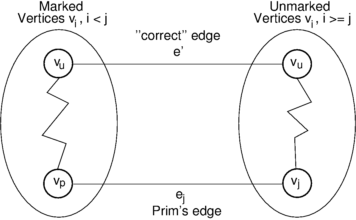
Figure 19.6.2: Prim’s MCST algorithm proof. The left oval contains that portion of the graph where Prim’s MCST and the “true” MCST \(\mathbf{T}\) agree. The right oval contains the rest of the graph. The two portions of the graph are connected by (at least) edges \(e_j\) (selected by Prim’s algorithm to be in the MCST) and \(e'\) (the “correct” edge to be placed in the MCST). Note that the path from \(v_w\) to \(v_j\) cannot include any marked vertex \(v_i, i \leq j\), because to do so would form a cycle.¶