
12.16. Array Implementation for Complete Binary Trees
12.16.1. Array Implementation for Complete Binary Trees
From the full binary tree theorem, we know that a large fraction of the space in a typical binary tree node implementation is devoted to structural overhead, not to storing data. This module presents a simple, compact implementation for complete binary trees. Recall that complete binary trees have all levels except the bottom filled out completely, and the bottom level has all of its nodes filled in from left to right. Thus, a complete binary tree of \(n\) nodes has only one possible shape. You might think that a complete binary tree is such an unusual occurrence that there is no reason to develop a special implementation for it. However, the complete binary tree has practical uses, the most important being the heap data structure. Heaps are often used to implement priority queues and for external sorting algorithms.
We begin by assigning numbers to the node positions in the complete binary tree, level by level, from left to right as shown in Figure 12.16.1. An array can store the tree’s data values efficiently, placing each data value in the array position corresponding to that node’s position within the tree. The table lists the array indices for the children, parent, and siblings of each node in Figure 12.16.1.
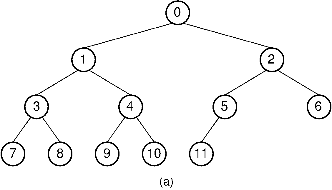
Figure 12.16.1: A complete binary tree of 12 nodes, numbered starting from 0.
Here is a table that lists, for each node position, the positions of the parent, sibling, and children of the node.
Looking at the table, you should see a pattern regarding the positions of a node’s relatives within the array. Simple formulas can be derived for calculating the array index for each relative of a node \(R\) from \(R\)’s index. No explicit pointers are necessary to reach a node’s left or right child. This means there is no overhead to the array implementation if the array is selected to be of size \(n\) for a tree of \(n\) nodes.
The formulae for calculating the array indices of the various relatives of a node are as follows. The total number of nodes in the tree is \(n\). The index of the node in question is \(r\), which must fall in the range 0 to \(n-1\).
Parent(\(r\)) \(= \lfloor(r - 1)/2\rfloor\) if \(r \neq 0\).
Left child(\(r\)) \(= 2r + 1\) if \(2r + 1 < n\).
Right child(\(r\)) \(= 2r + 2\) if \(2r + 2 < n\).
Left sibling(\(r\)) \(= r - 1\) if \(r\) is even and \(r \neq 0\).
Right sibling(\(r\)) \(= r + 1\) if \(r\) is odd and \(r + 1 < n\).