
23.4. Finding the \(i\) th Best Element
We now tackle the problem of finding the \(i\) th best element in a list. Is this easier or harder than finding the max and second biggest? Is this easier or harder than finding the max and the min? On the one hand, it is only one element. On the other hand, it seems like it could be a “harder” element to locate.
One solution is to sort the list and simply look in the \(i\) th position. However, this process provides considerably more information than we need to solve the problem. So intuitively, it seems to be less efficient than what is might be possible. The minimum amount of information that we actually need to know can be visualized as shown in Figure 23.4.1. That is, all we need to know is the \(i-1\) items less than our desired value, and the \(n-i\) items greater. We do not care about the relative order within the upper and lower groups. So can we find the required information faster than by first sorting? Looking at the lower bound, can we tighten that beyond the trivial lower bound of \(n\) comparisons? We will focus on the specific question of finding the median element (i.e., the element with rank \(n/2\)), because the resulting algorithm can easily be modified to find the \(i\) th largest value for any \(i\).
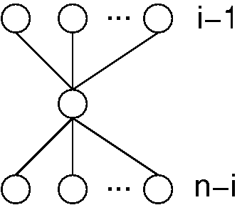
Figure 23.4.1: The poset that represents the minimum information necessary to determine the \(i\) th element in a list. We need to know which element has \(i-1\) values less and \(n-i\) values more, but we do not need to know the relationships among the elements with values less or greater than the \(i\) th element.
Looking at the Quicksort algorithm might give us some insight into solving the median problem. Recall that Quicksort works by selecting a pivot value, partitioning the array into those elements less than the pivot and those greater than the pivot, and moving the pivot to its proper location in the array. Partitioning the array costs \(O(n)\) comparisons. If the pivot is in position \(i\), then we are done. If not, we can solve the subproblem recursively by only considering one of the sublists. That is, if the pivot ends up in position \(k > i\), then we simply solve by finding the \(i\) th best element in the left partition. If the pivot is at position \(k < i\), then we wish to find the \(i-k\) th element in the right partition.
What is the worst case cost of this algorithm? As with Quicksort, we get bad performance if the pivot is the first or last element in the array. This would lead to possibly \(O(n^2)\) performance. However, if the pivot were to always cut the array in half, then our cost would be modeled by the recurrence \(\mathbf{T}(n) = \mathbf{T}(n/2) + n = 2n\) or \(O(n)\) cost.
Finding the average cost requires us to use a recurrence with full history, similar to the one we used to model the cost of Quicksort. If we do this, we will find that \(\mathbf{T}(n)\) is in \(O(n)\) in the average case.
Is it possible to modify our algorithm to get worst-case linear time? To do this, we need to pick a pivot that is guaranteed to discard a fixed fraction of the elements. We cannot just choose a pivot at random, because doing so will not meet this guarantee. The ideal situation would be if we could pick the median value for the pivot each time. But that is essentially the same problem that we are trying to solve to begin with.
Notice, however, that if we choose any constant \(c\), and then if we pick the median from a sample of size \(n/c\), then we can guarantee that we will discard at least \(n/2c\) elements. Actually, we can do better than this by selecting small subsets of a constant size (so we can find the median of each in constant time), and then taking the median of these medians. Figure 23.4.2 illustrates this idea.
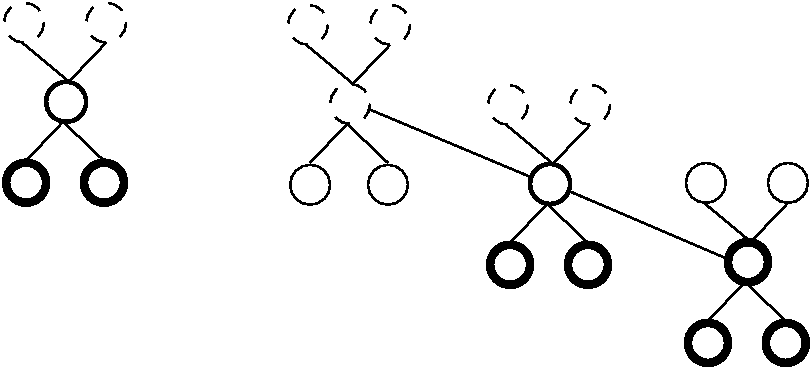
Figure 23.4.2: A method for finding a pivot for partitioning a list that guarantees at least a fixed fraction of the list will be in each partition. We divide the list into groups of five elements, and find the median for each group. We then recursively find the median of these \(n/5\) medians. The median of five elements is guaranteed to have at least two in each partition. The median of three medians from a collection of 15 elements is guaranteed to have at least five elements in each partition.
This observation leads directly to the following algorithm.
Choose the \(n/5\) medians for groups of five elements from the list. Choosing the median of five items can be done in constant time.
Recursively, select \(M\), the median of the \(n/5\) medians-of-fives.
Partition the list into those elements larger and smaller than \(M\).
While selecting the median in this way is guaranteed to eliminate a fraction of the elements (leaving at most \(\lceil (7n - 5)/10\rceil\) elements left), we still need to be sure that our recursion yields a linear-time algorithm. We model the algorithm by the following recurrence.
The \(\mathbf{T}(\lceil n/5 \rceil)\) term comes from computing the median of the medians-of-fives, the \(6\lceil n/5 \rceil\) term comes from the cost to calculate the median-of-fives (exactly six comparisons for each group of five elements is needed), and the \(\mathbf{T}(\lceil (7n - 5)/10\rceil)\) term comes from the recursive call of the remaining (up to) 70% of the elements that might be left.
We will prove that this recurrence is linear using the process of constructive induction. We assume that it is linear for some constant \(r\), and then show that \(\textbf{T}(n) \leq rn\) for all \(n\) greater than some bound.
We might need to hunt around a bit to find values for \(r\) and \(n\) that make this equation work. For example, if we try \(r = 1\) then we get \(3.1 n + 7.5 \leq n\) which clearly does not work. But if we use \(r = 23\) we get \(22.9n + 39.5 \leq 23n\), which is true for \(n \geq 395\). This provides a base case that allows us to use induction to prove that \(\forall n \geq 395, \mathbf{T}(n) \leq 23n\).
While we have now proved that the median (or \(i\) th element) can be done in linear time, in reality this algorithm is not practical because its constant factor costs are so high. So much work is being done to guarantee linear time performance that it is more efficient on average to rely on chance to select the pivot, perhaps by picking it at random or picking the middle value out of the current subarray.
23.4.1. Acknowledgement
This page borrows heavily from presentation in Section 3.5 of Compared to What? by Gregory J.E. Rawlins.